image =	frequencyFiltering2dImg (inImg,frequencyBandPassFilterType,cutoffFrequency,inStdDev)
image =	frequencyFiltering2dImg (inImg,frequencyBandPassFilterType,cutoffFrequency,inStdDev,theta,thetaRange)

Detailed Description

Filters an image in Fourier domain by selecting a frequency range.

This algorithm applies a band-pass filter to the input image in the frequency domain. Such an approach is very powerful since a convolution in the spatial domain becomes a pixelwise multiplication in the Fourier domain. Hence, it is computationnally faster than a spatial filtering, in particular for large kernel sizes. Moreover, it is possible to design a filter in order to fit a determined frequency range.

The steps of the algorithm are:

Compute $I=\lbrace I_{Real}, I_{Imag} \rbrace$ , the disctrete Fourier transform of the input image,
Multiply each element of $I_{Real}$ and $I_{Imag}$ by its related filter coefficient,
Compute the inverse discrete Fourier transform of ,
In order to keep the same buffer type, the output of the inverse Fourier transform (which has initially Real32 data type) is converted.

The figure below illustrates how the band-pass filtering in frequency domain works (the signal spectrum is normalized for convenience).

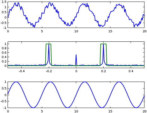
The first row displays a noisy signal, which normalized frequency equals 0.2. In the second row are shown the signal spectrum and a window filter centered around 0.2 (the signal frequency). Because the signal spectrum is symmetric, so is the filter. Finally, the third row plots the reconstructed signal: the noise has been deleted.

However, a step filter as illustrated in the figure above will produce ringing artefacts (https://en.wikipedia.org/wiki/Ringing_artifacts), as shown in the figure below:

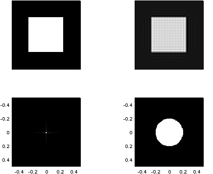
In this figure, the initial image is a square (top-left image), its spectrum modulus (bottom-left image), the filter (bottom-right image) and the resulting filtered image, presenting ringing artefacts (top-right image).

For this reason, the algorithm does not use window filters and two other band-pass filters instead:

Gaussian band-pass filter
$F(f) = e^{-\frac{ \left( f - f_0 \right)^2}{2 \sigma^2}}$
LogGabor band-pass filter
$F(f) = e^{-\frac{ \left( \log \left( f / f_0 \right) \right)^2}{2 \left( \log \left( \sigma / f_0 \right) \right)^2}}$

where $f = \sqrt{u^2+v^2}$ , $u, v$ being respectively the frequencies along the image axes.

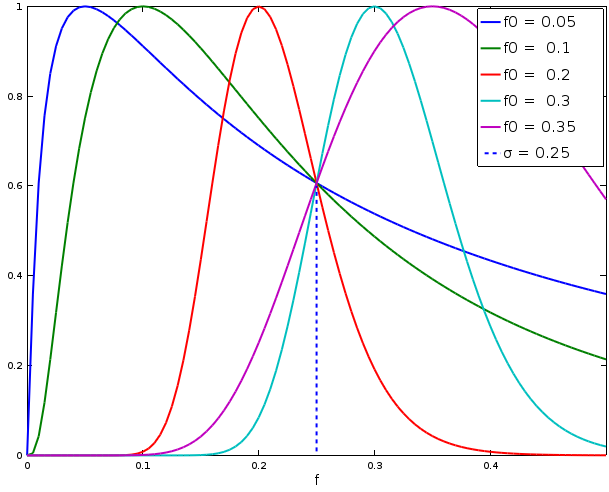
Both filters need only two parameters: a cutoff frequency cutoffFrequency and a standard deviation stdDev, which make them easily configurable. However, the logGabor bandwidth changes when varying the cutoff frequency, even if the standard deviation is constant. The figure below shows how the logGabor function varies when the cut off frequency increases and the standard deviation is constant and set to 0.25.

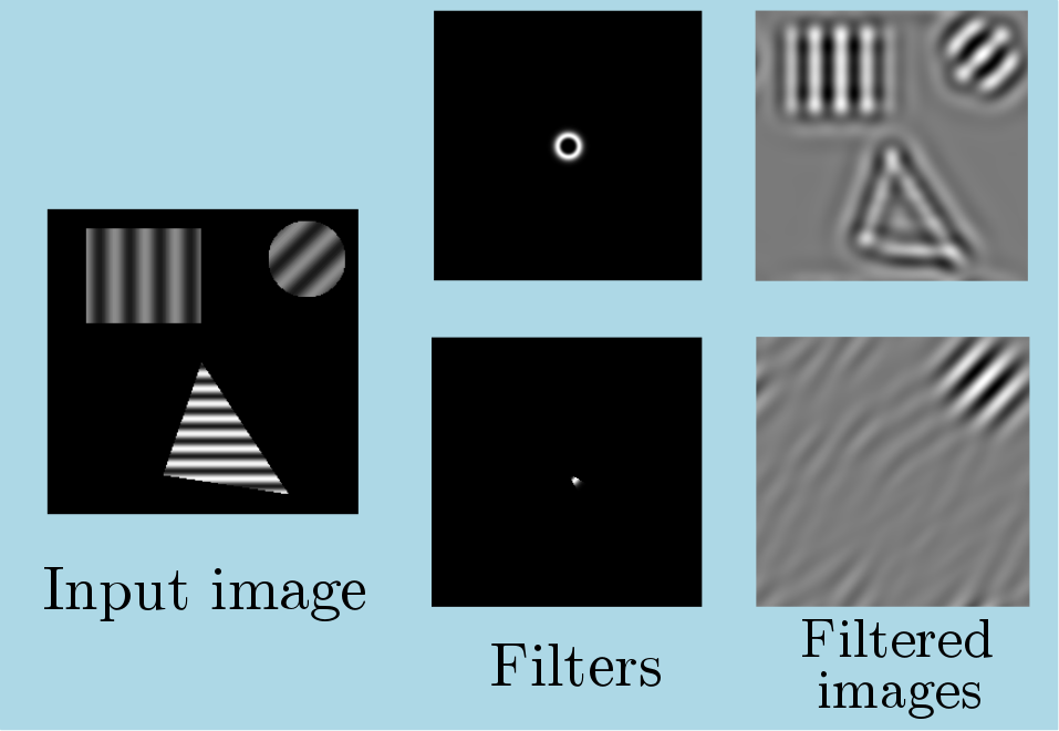
In some images, it may be interesting to isolate a texture with a specific orientation. For this reason, the algorithm allows to specify an orientation theta and a range thetaRange which will mask the filtered spectrum and keep only the information in the desired direction range, both in degrees.

Note: We must have 0° $\leq$ theta $\leq$ 180° and 0° < thetaRange $\leq$ 180°. If not, the default values are theta = 0° and thetaRange = 180° (i.e. select all the orientations).

The figure below illustrates an image with three shapes in the first column. The square and the circle textures have the same frequency (0.04) but different orientations whereas the triangle texture frequency is different (0.08). The second columns shows the logGabor filter configured to select the square and circle textures (top) and its masked oriented version (bottom). Finally, the third column displays the resulting filtered images. We can see that both textures are selected in the non oriented filter whereas only the texture of the circle remains after applying the oriented filter.

Note: There is a subtlety between orientation of the texture and the spectrum. A horizontal spreading sinusoid yields vertical strips, as shown in the top-left figure below. That is why the spectrum is oriented horizontally. The filter orientation is hence 0° and not 90°. In the same way, the sinusoid and its spectrum in the second row have an orientation of 30° (clockwise) but the texture apprears like 60° (counter-clockwise) oriented strips.

Example of Python code :

Example imports

import PyIPSDK

import PyIPSDK.IPSDKIPLFiltering as filter

Code Example

    # opening of input images
    inImg = PyIPSDK.loadTiffImageFile(inputImgPath)
    
    # define the parameters
    f0 = 0.2
    sigma = 0.18
    theta = 45
    thetaRange = 30
    
    # Gaussian Band-pass filtering
    outGaussianImg = filter.frequencyFiltering2dImg(inImg, PyIPSDK.eFrequencyBandPassFilterType.eFBPFT_Gaussian, f0, sigma, theta, thetaRange)
    # LogGabor Band-pass filtering
    outLogGaborImg = filter.frequencyFiltering2dImg(inImg, PyIPSDK.eFrequencyBandPassFilterType.eFBPFT_LogGabor, f0, sigma, theta, thetaRange)

Example of C++ code :

Example informations

Header file

#include <IPSDKIPL/IPSDKIPLFiltering/Processor/FrequencyFiltering2dImg/FrequencyFiltering2dImg.h>

Code Example

        // Gaussian frequency filtering
        // -----------------------------------
        ImagePtr pGaussOutImg = frequencyFiltering2dImg(pInImg, eFrequencyBandPassFilterType::eFBPFT_Gaussian, f0, sigma, theta, thetaRange);
        // LogGabor frequency filtering
        // -----------------------------------
        ImagePtr pLogGaborOutImg = frequencyFiltering2dImg(pInImg, eFrequencyBandPassFilterType::eFBPFT_LogGabor, f0, sigma, theta, thetaRange);