Introduction

Some image processing algorithms, such as convolution or mean smoothing algorithms, compute the result for each pixel according to a local neighbourhood $\aleph$ . Since the whole neighbourhood is known, such calculation is not an issue for pixels with coordinates $x_i \geq halfKnlSize_i$ and $x_i < ImSize_i-halfKnlSize_i$ , where $halfKnlSize_i$ and $ImSize_i$ are respectively the half size of $\aleph$ and the image size along the direction $i \in \lbrace x, y, z, c, t \rbrace$ and $x_i$ is the pixel coordinate along this direction. However, for pixels on the borders of the image, some information is missing (see the figure below).

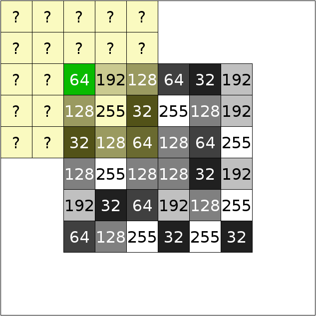
Process for the top-left pixel of the image (in green), the algorithm needs its 5x5 neighbourhood, but 16 values are unknown.

In order to process these pixels, the algorithm has to determine the values of the pixels out of the image. For this, one of the following hypothesis is necessary:

the pixels out of the image have a specific value,
the pixels out of the image have the same value than the pixel on the border of the image,
the pixels out of the image simulates a mirror of the image.

Classical border policy types

Specific value

The first type of border policy is ipsdk::image::valuedBorder2d.

It defines a border policy with a specific value. It can be used to set a neutral value to the pixels out of the image. For example, this value can be set to 0 when computing a sum along the pixel's local neighbourhood.

Note: It can also be useful to compute the local minimum or maximum. In these cases, ipsdk::image::valuedMinBorder2d() and ipsdk::image::valuedMaxBorder2d() can be called to directly assign the minimum or maximum value possible according to the image buffer type.

The following figure illustrates the case that the pixels out of the image have been initialize with zero values (only the pixels inside the kernel are represented). This way, calculating the sum along the kernel will only take into account the values inside the image: 64+192+128+128+64+32+32+128+64 = 832.

The pixels out of the image have zero value. Only the pixels inside the kernel are represented.

The following Python sample loads an image and computes a convolution with a valued border policy initializing the pixels out of the image with 0 values:

# Import the needed IPSDK modules
import PyIPSDK
import PyIPSDK.IPSDKIPLFiltering as filter
# Define the input image path
# ...
# Load the input image
im = PyIPSDK.loadTiffImageFile(inputPath)
# Define the kernel
inKnl = PyIPSDK.rectangularKernelXY(1, 2, [1.5, 1.2, 1.4,
                                           4.2, 7.0, 2.3,
                                           3.5, 4.8, 7.5,
                                           1.9, 2.3, 6.3,
                                           9.5, 0.2, 4.1])
# Define the border policy
borderPolicy = PyIPSDK.valuedBorder2d(0);
#Compute the convolution
res = filter.convolution2dImg(im, inKnl, True, borderPolicy)

The C++ code equivalent to the previous python script is:

// used to initialize IPSDK environment
#include <IPSDKCore/Config/LibraryInitializer.h>
// used to compute the convolution
#include <IPSDKIPL/IPSDKIPLFiltering/Processor/Convolution2dImg/Convolution2dImg.h>
// used for border policy
#include <IPSDKImage/Fragment/BorderPolicy/2d/Border2dPolicyUtils.h>
// used to define the convolution kernel
#include <IPSDKBaseData/Pattern/Kernel/KernelXY.h>
#include <IPSDKBaseData/Pattern/OffsetXY.h>
// used to read/write an image from/to a TIFF file:
#include <IPSDKImageFile/Tiff/TiffImageFileUtils.h>
int main(int argc, char* argv[])
{
    // Define the input image path
    // ...
    
    // Load the input image
    ImagePtr pImg = ipsdk::image::file::loadTiffImageFile(inputPath);
    // Define the kernel
    KernelXYPtr pInKnlXY(boost::make_shared<KernelXY>());
    pInKnlXY->insert(OffsetXY(-1, -2), 1.5f);
    pInKnlXY->insert(OffsetXY(0, -2), 1.2f);
    pInKnlXY->insert(OffsetXY(1, -2), 1.4f);
    pInKnlXY->insert(OffsetXY(-1, -1), 4.2f);
    pInKnlXY->insert(OffsetXY(0, -1), 7.0f);
    pInKnlXY->insert(OffsetXY(1, -1), 2.3f);
    pInKnlXY->insert(OffsetXY(-1, 0), 3.5f);
    pInKnlXY->insert(OffsetXY(0, 0), 4.8f);
    pInKnlXY->insert(OffsetXY(1, 0), 7.5f);
    pInKnlXY->insert(OffsetXY(-1, 1), 1.9f);
    pInKnlXY->insert(OffsetXY(0, 1), 2.3f);
    pInKnlXY->insert(OffsetXY(1, 1), 6.3f);
    pInKnlXY->insert(OffsetXY(-1, 2), 9.5f);
    pInKnlXY->insert(OffsetXY(0, 2), 0.2f);
    pInKnlXY->insert(OffsetXY(1, 2), 4.1f);
    // Define the border policy
    Border2dPolicyPtr pBorder2dPolicy = ipsdk::image::valuedBorder2d(0);
    // Compute the convolution
    ImagePtr pOutImg = ipsdk::imaproc::filter::convolution2dImg(pImg, pInKnlXY, true, pBorder2dPolicy);
    
    return 0;
}

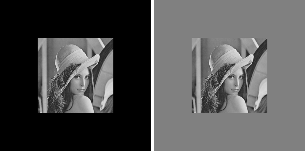
The following figure illustrates two examples of value border policy on the image of Lena. The first one initializes the pixels out of the image to 0 whereas the second initializes them to 128.

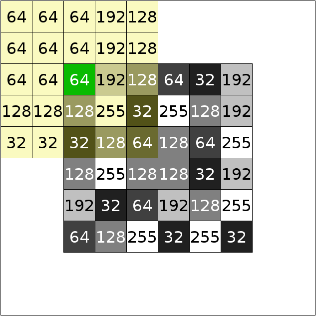
Examples of value border policy. The values were set to 0 (left) and 128 (right).

Continue value

The second type of border policy is ipsdk::image::continueBorder2d.

With this border policy, the pixels out of the image will have the same value than the pixel along the border of the image, as shown in the following figure:

The pixels out of the image have the same value than the pixels in the border of the image. Only the pixels inside the kernel are represented.

The followong command shows how to build a continue border policy in python. This instruction replaces the line 19 in the first sample:

borderPolicy = PyIPSDK.continueBorder2d();

The equivalent C++ code is:

Border2dPolicyPtr pBorder2dPolicy = ipsdk::image::continueBorder2d();

The following figure illustrates the continue border policy on the image of Lena.

Example of continue border policy.

Mirror effect

The third type of border policy is ipsdk::image::mirorBorder2d.

With this border policy, the pixels out of the image will simulate a mirror effect of the image. Two kinds of mirror effect exist:

with duplication of the pixel along the border. Considering negative indices for pixels out of the image ( is the first pixel inside the image), we can express the copy by . In this case, we will obtain , , etc. This is the mirror policy used by IPSDK.
without duplication of the pixel along the border. Considering negative indices for pixels out of the image ( is the first pixel inside the image), we can express the copy by . In this case, we will obtain , , etc.

Illustration of the mirror effect border policy used by IPSDK. Only the pixels inside the kernel are represented.

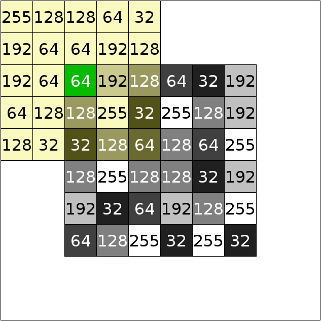
The followong example shows how to build a mirror border policy in python. This instruction replaces the line 19 in the first sample:

borderPolicy = PyIPSDK.mirorBorder2d();

The equivalent C++ code is:

Border2dPolicyPtr pBorder2dPolicy = ipsdk::image::mirorBorder2d();

The following figure illustrates the mirror border policy on the image of Lena.

Example of mirror border policy.