image =	localHistogramModule2dImg (inImg,inHalfKnlSizeX,inHalfKnlSizeY)
image =	localHistogramModule2dImg (inImg,inHalfKnlSizeX,inHalfKnlSizeY,inOptNbClasses)

Detailed Description

Lowitz local histogram module on a 2d image.

This algorithm computes for each pixel of the output image its associated local histogram module, as defined by Lowitz [1], on a rectangular neighbourhood.

This measure is the difference between the actual local histogram $H$ and the theoretical histogram $H_t$ for which each bin has the same value. This difference is calculated by the Mahalanobis distance and can be expressed as :

$d(H, H_t) = \sum_{i = 0}^{C-1}{\frac{\vert E(H_i) - E(H_{ti}) \vert}{\sqrt{\sigma^2(H_i) + \sigma^2(H_{ti})}}}$

Where $C$ is the number of classes in the histogram, $E(H_i)$ is the expected value of the $i^{th}$ bin of the histogram $H$ and $\sigma^2(H_i)$ is its variance.

We define $p_i$ as the value of the normalized histogram : $p_i = \frac{H_i}{N}$ , with $N = N_x \times N_y = \sum_{i = 0}^{C-1}{H_i}$ being the number of pixels in the neighbourhood.

Since this measure is based on Bernoulli distribution, the expected value of $H_i$ and its variance are :

$E(H_i) = p_i$

$\sigma^2(H_i) = p_i \left( 1-p_i \right)$

Moreover the theoretical histogram $H_t$ has the following expected value (and hence probability) and variance for each bin :

$E(H_{ti}) = \frac{1}{C}$

$\sigma^2(H_{ti}) = \frac{1}{C} \left( 1 - \frac{1}{C} \right)$

With $N$ draws (1 per pixel in the neighbourhood), we can rewrite the Mahalanobis distance as follows :

$\begin{eqnarray*} d(H, H_t) & = & \sum_{i = 0}^{C-1}{\frac{\vert N p_i - \frac{N}{C} \vert}{\sqrt{N p_i \left( 1 - p_i \right) + \frac{N}{C} \left( 1 - \frac{1}{C} \right)}}} \\ & = & \sum_{i = 0}^{C-1}{\frac{\vert H_i - \frac{N}{C} \vert}{\sqrt{H_i \left( 1 - p_i \right) + \frac{N}{C} \left( 1 - \frac{1}{C} \right)}}} \end{eqnarray*}$

The histogram $H$ is computed on the rectangular kernel, with the following parameters:

number of classes = ,
$min_{histo}$ = minimum value of the whole input image,
$max_{histo}$ = maximum value of the whole input image.

The number of classes is an optional parameter of the algorithm. Its default value equals to 16. If the number of classes specified by the user exceeds the maximum allowed number of classes given the input image data type and dynamic range, it is automatically adjusted. For instance:

a number of classes initialized to value 16 will be automatically adjusted to value 2 for a binary input image,
a number of classes initialized to value 256 will be automatically adjusted to value 10 for a integral input image whose dynamic range equals to .

The borders of the input image are handled by padding pixels with a mirror reflection of the border pixels in the input image (see Border policy for more details).

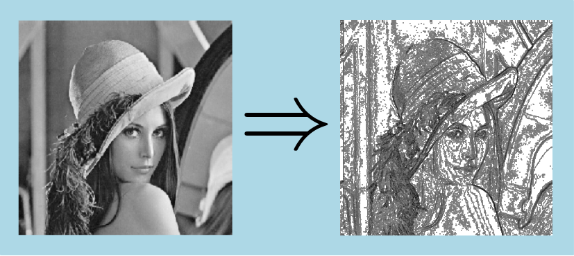
Here is an example of an output image computed from the LocalHistogramModule2dImg algorithm on a 8-bits grey level, with a kernel of size 3x3 pixels and 16 classes:

References

[1] G. Lowitz "Can a Local Histogram Really Map Texture Information?". Pattern Recognition, 16, 2, 1983, pp 141–147.

Example of Python code :

Example imports

import PyIPSDK

import PyIPSDK.IPSDKIPLStats as stats

Code Example

    # opening of input image
    inImg = PyIPSDK.loadTiffImageFile(inputImgPath)
    
    # local entropy 2d image computation
    outImg = stats.localHistogramModule2dImg(inImg, 3, 3)

Example of C++ code :

Example informations

Header file

#include <IPSDKIPL/IPSDKIPLStats/Processor/LocalHistogramModule2dImg/LocalHistogramModule2dImg.h>

Code Example

// compute local energy on input image

ImagePtr pOutImg = localHistogramModule2dImg(pInImg, inHalfKnlSizeX, inHalfKnlSizeY, nbClasses);