 |
IPSDK 4.2
IPSDK : Image Processing Software Development Kit
|
|
IPSDK 4.2
IPSDK : Image Processing Software Development Kit
|
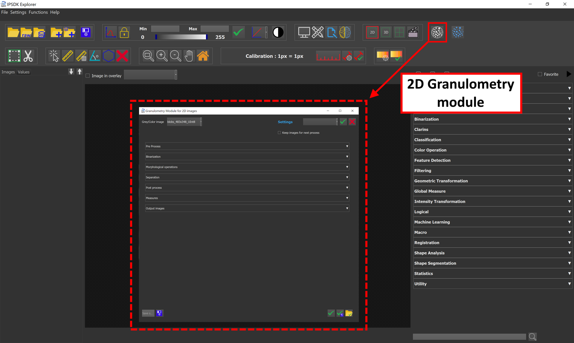
The 2D Granulometry [1] module is designed to detect, separate, and analyze grains in 2D. It is accessible via one dedicated button, inside the menu bar of IPSDK Explorer.
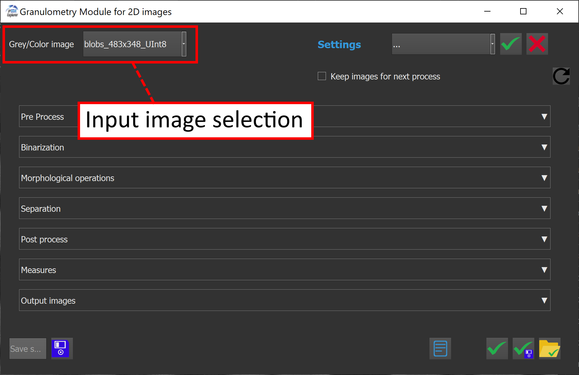
The module window contains a dropdown menu at the top left corner to select an input image to process. Both grayscale and RGB formats are supported, for individual 2D images or sequences of 2D images.
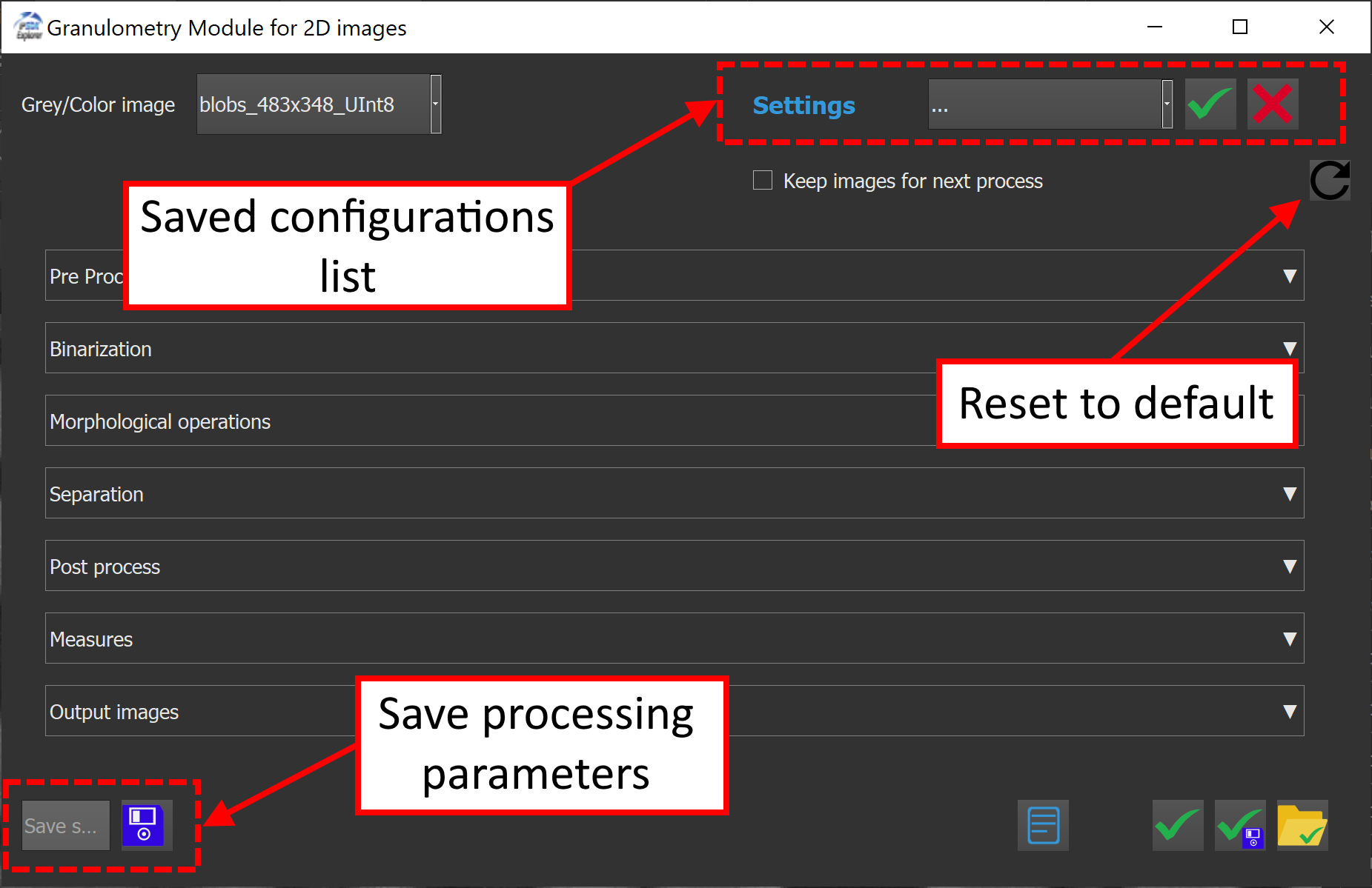
The second dropdown menu appearing on the right corner allows to choose and reload previously saved configurations. The special entry "..." refers to the last auto-saved configuration made during the last preview.
| Buttons | Description |
|---|---|

| Apply the settings to the different processing sections |

| Delete the current setting selected in the list |

| Import saved settings |

| Export saved settings |

| Save current configuration |

| Reset all the settings to default values |
The checkbox Keep images for next process is an optional setting that allows to keep processed images in memory for the next process, and therefore gain some time during computations. When this option is checked, the last previewed image will be saved in memory, reducing redundant computations.
To save the current configuration :
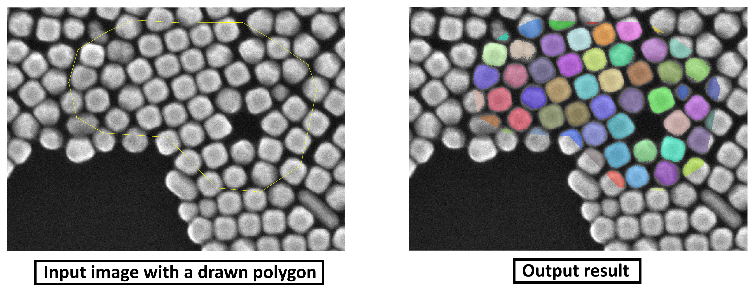
The plugin allows to create masks before processing the image, in order to specify a Region Of Interest (ROI) where the processing will be applied. Masks can be defined using the polygon tool available in the menu bar of IPSDK Explorer.
Each click within the viewer adds a new point to the polygon, while a double-click closes the shape. The polygon can be further adjusted after creation using the selection tool and repositioning the different points of the polygon.
Once the editing has been finished, the corresponding mask will be applied to the final result or inside the previews.
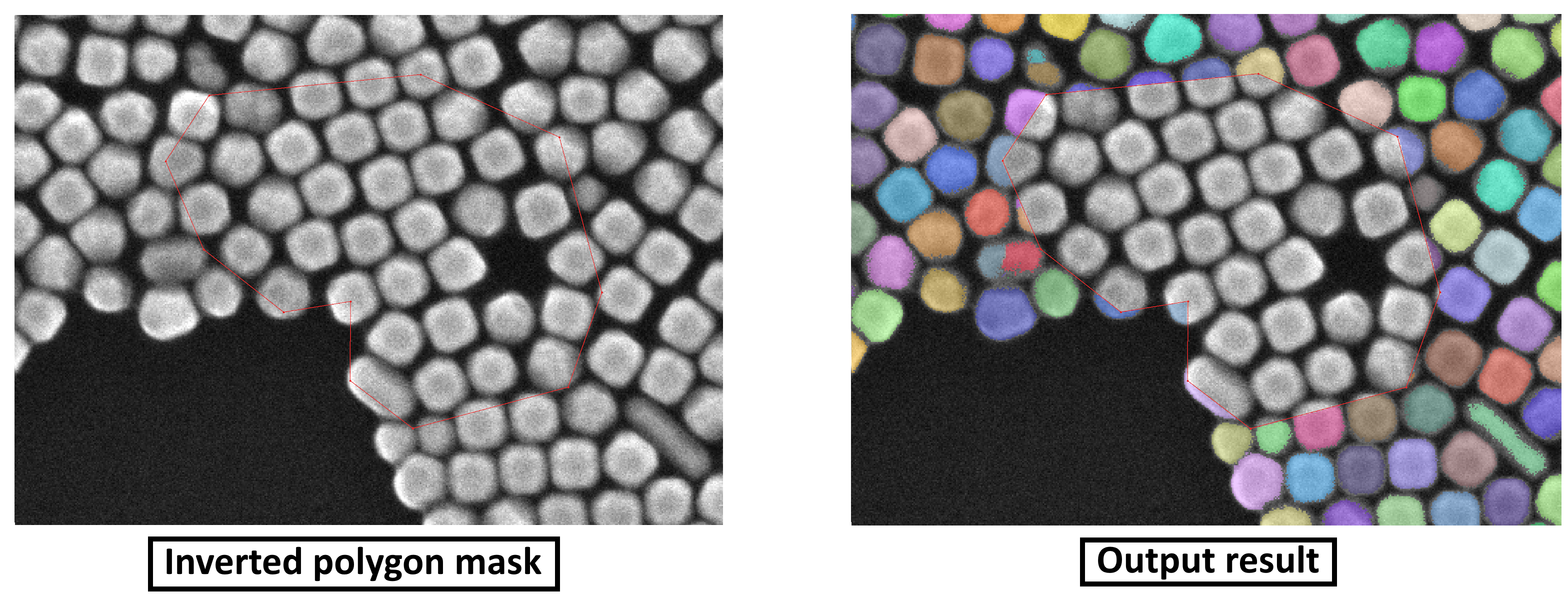
It is also possible to define exclusion regions within the mask, in order to omit specific areas from the segmentation result.
There are two different ways to use inverted polygons. First, they can be used to exclude specific regions from the result image.
They can also be combined with standard polygons to create masks with internal holes.
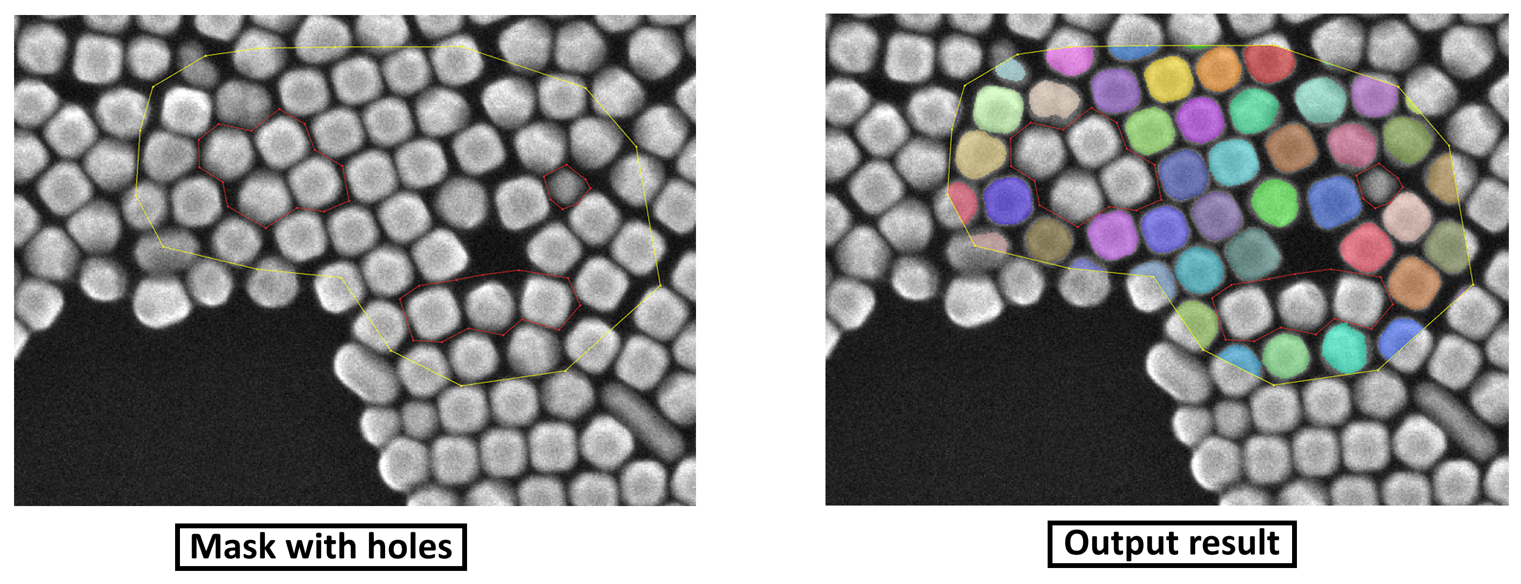
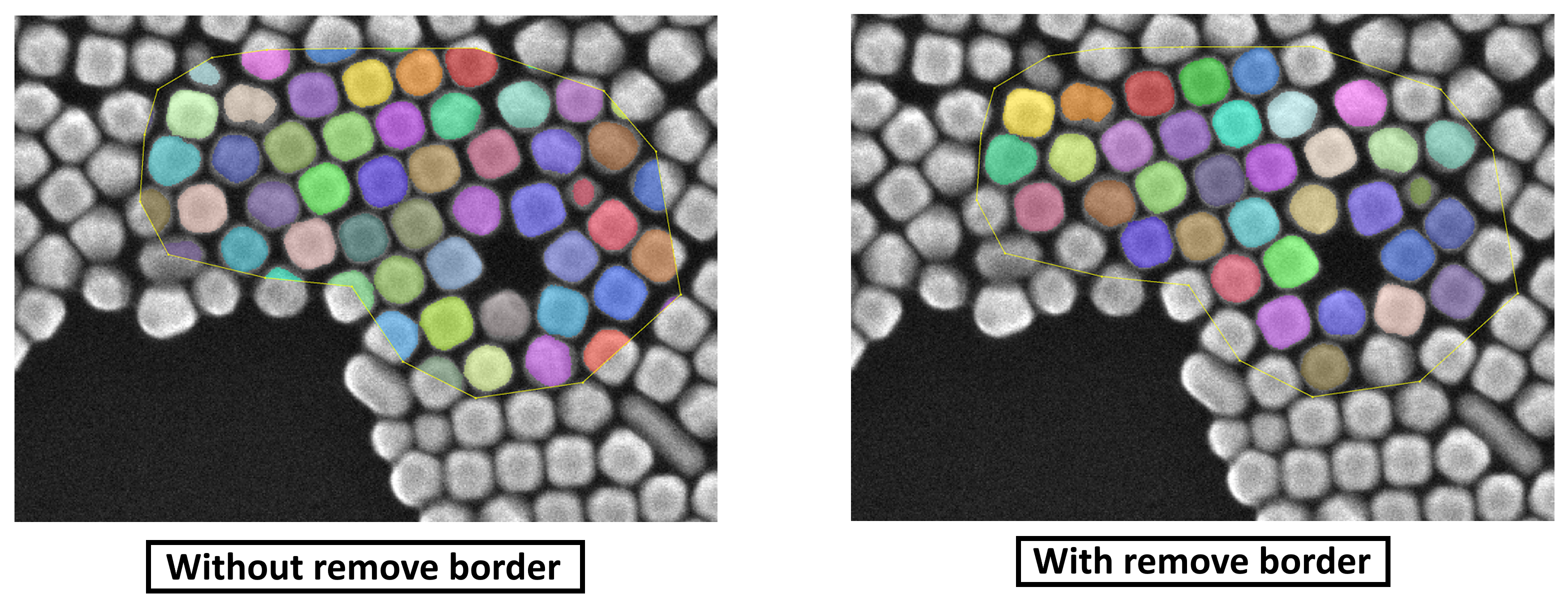
Additionally, the remove border function, available in the post process section, can be used to remove objects that intersect the mask boundaries.
The core of the plugin window includes seven distinct and collapsible processing sections :
Each processing section is made up of individual functions.
Each line is described as follows :

Here is an example with the pre process section :

This section is intended to enhance image quality before grain detection.
It includes:
Here's an example of pre processing :

This step converts the pre-processed image into a binary mask highlighting the grains.
This section includes 5 thresholding methods, with 3 classical algorithms :
And also two advanced options :

Here is an example of a binarization using the Simple threshold method :


After clicking the edit button, a new window opens allowing to choose a threshold using the double slider at the bottom of the window.

When using the smart segmentation method, a pre-trained model is needed. The documentation shows how to build a smart segmentation model here.
The smart segmentation option allows to select a pre-trained model and to choose the model classes to use for the binarization.
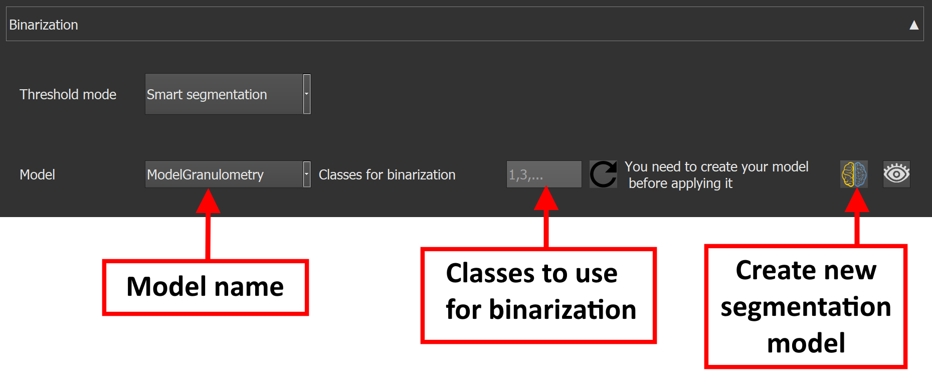
Here is an example of binarization using the smart segmentation method :

Besides the smart segmentation algorithm, the macro-based binarization can be usefull for very complex images binarization.
The previous example shows that the binarization isn't perfect with a multitude of holes inside the objects. To improve the binary image we can use morphological operations.
Morphological operations refine the binary image by cleaning up artifacts and enhancing the separation of grains.
Available operations are :
Each operation is optional and configurable.
Here's an example of holes removal using the morphological operations inside the module :

Grain segmentation is performed here to label individual grains for further analysis.
Three different segmentation methods are available :
Only one method can be selected at a time.

Additional cleaning of the labeled result can be performed here using a set of post-processing tools.
This section implements 4 different methods :
Here is an example of post process :

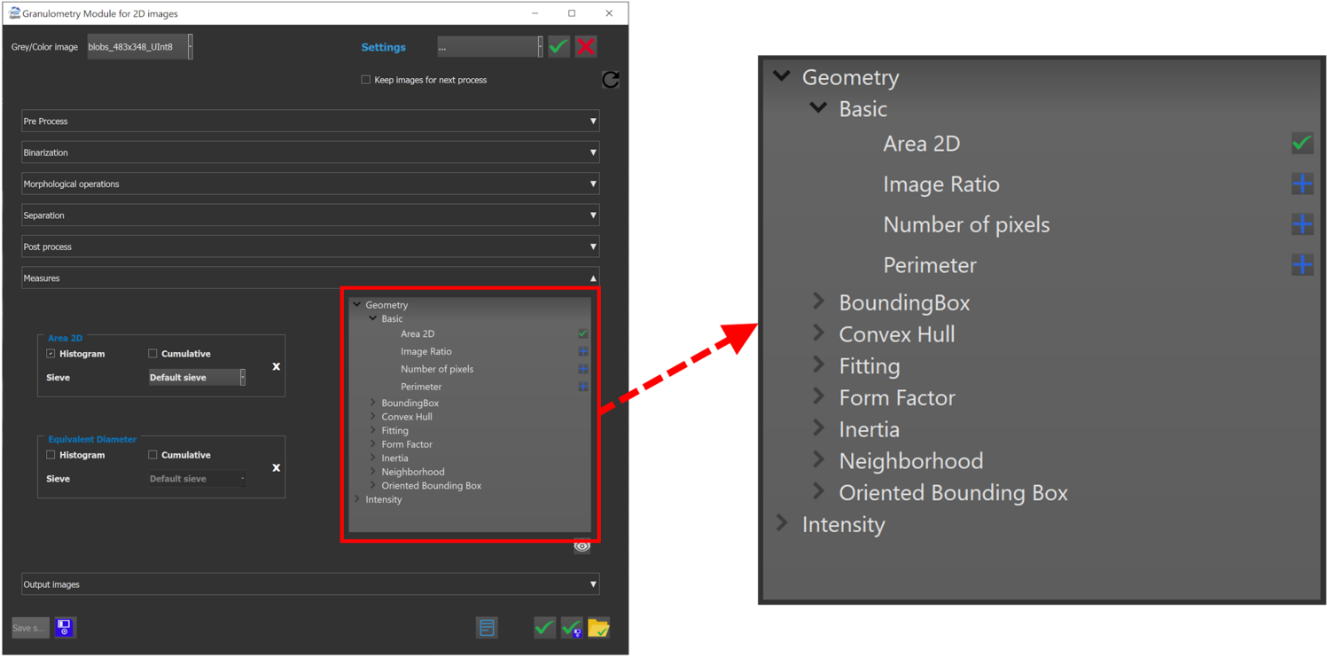
This section provides quantitative analysis of the segmented grains.
It is divided in two different parts :
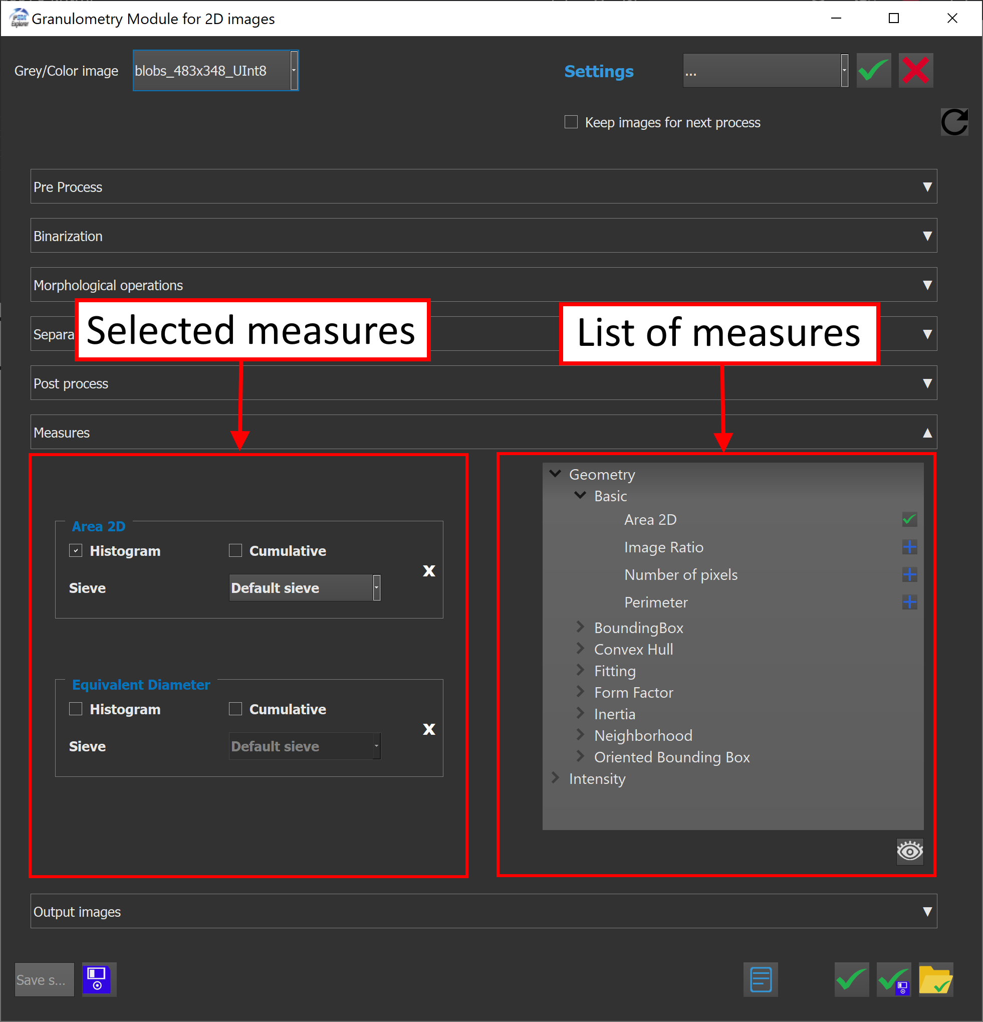
The right pane lists all available measurements.

The preview button gives a peak of the results inside IPSDK Explorer.
Once a measure is added, it appear on the left side with the possibility to compute two histograms by clicking the checkboxes.
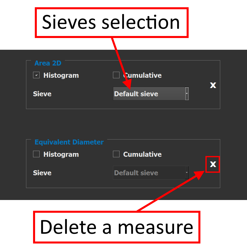
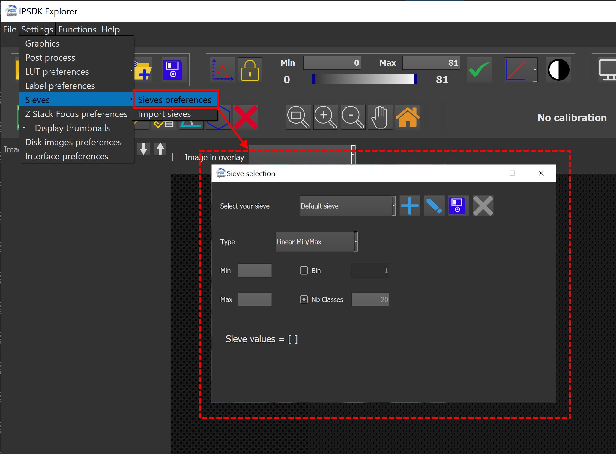
Sieves can be customized under Settings → Sieves → Preferences.
This section defines the type of output results (label images, binary masks, overlays, etc.) to compute and save.
| Output type | Description | Example |
|---|---|---|
| Label image | Returns a label image of the segmented grains | 
|
| Color image | Returns the label image as a RGB image | 
|
| Merge input and color image | Returns the input image blended with the label image in overlay | 
|
| Input image with contours | Returns the input image blended with the contours of the labels in overlay | 
|
At the bottom right, three buttons control the execution of the analyses :


Here's an example of display inside IPSDK Explorer when launching an analysis :


[1] https://en.wikipedia.org/wiki/Granulometry
[2] https://en.wikipedia.org/wiki/Watershed_(image_processing)
